

Field Comparisons Using Snowflake
Use cases for bulk field comparisons
There are a lot of reasons why it may be necessary to compare the values of some but not all fields in two tables. In billing reconciliation, one table may contain raw line items, and another table may contain lines in billing statements. Another common reason would be to verify that fields are accurate after undergoing transformation from the source system to a table optimized for analytics.
Obviously when moving and transforming data a lot can happen along the way. Probably the most common problem is missing rows, but there are any number of other problems: updates out of sync, data corruption, transformation logic errors, etc.
How to compare fields across tables in Snowflake
Fortunately, Snowflake’s super-fast table joining provides a great way to check for missing rows or differences in key fields between the tables. Without getting into Venn diagrams with inner, outer, left, right, etc., suffice it to say we’re going to discuss what is perhaps the least used join: the full outer exclusive of inner join. I’ve seen this type of join called other names, but this is what it does:
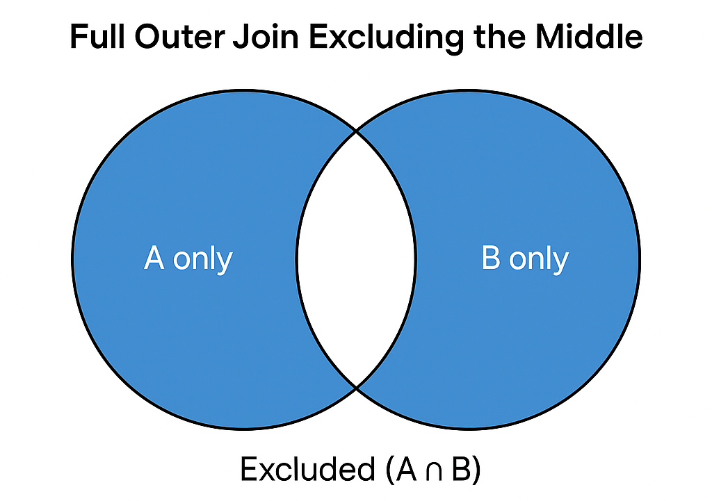
Think of it this way for the present use case: The excluded inner join excludes the rows with key fields that compare properly. In other words, if our reconciliation process on key fields between tables A and B is perfect, an inner join will return all rows. Turning that on its head, the inverse of an inner join (a full join exclusive of inner join) will return only the rows that have key field compare mismatches.
Snowflake performance for massive-scale field comparisons
The TPCH Orders tables used as a source has 150 million rows in it. Using this approach to compare four field values on 150 million rows, the equivalent of doing 600 million comparisons completed in ~12 seconds on an extra large cluster. This level of performance exceeds by orders of magnitude typical approaches such as using an ETL platform to perform comparisons and write a table of mismatched rows.
We can see how this works in the following Snowflake worksheet:
-- Set the context
use warehouse TEST;
use database TEST;
create or replace schema FIELD_COMPARE;
use schema FIELD_COMPARE;

-- Note: This test goes more quickly and consumes the same number of credits by temporarily
--       scaling the TEST warehouse to extra large. The test takes only a few minutes.
--       Remember to set the warehouse to extra small when done with the table copies and query.
--       The test will work on an extra small warehouse, but it will run slower and consume the
--       same number of credits as running on an extra large and finishing quicker.
alter warehouse TEST set warehouse_size = 'XLARGE';

-- Get some test data, in this case 150 million rows from TPCH Orders
create table A as select * from SNOWFLAKE_SAMPLE_DATA.TPCH_SF100.ORDERS;
create table B as select * from SNOWFLAKE_SAMPLE_DATA.TPCH_SF100.ORDERS;

-- Quick check to see if the copy looks right.
select * from A limit 10;
select * from B limit 10;

-- We will now check to be sure the O_ORDERKEY, O_CUSTKEY, O_TOTALPRICE, and O_ORDERDATE fields
-- compare properly between the two tables. The query result will be any comparison problems.
-- Because we have copied table A and B from the same source, they should be identical. We expect
-- That the result set will have zero rows.
select A.O_ORDERKEY      as A_ORDERKEY,
       A.O_CUSTKEY       as A_CUSTKEY,
       A.O_ORDERSTATUS   as A_ORDERSTATUS,
       A.O_TOTALPRICE    as A_TOTALPRICE,
       A.O_ORDERDATE     as A_ORDERDATE,
       A.O_ORDERPRIORITY as A_ORDERPRIORITY,
       A.O_CLERK         as A_CLERK,
       A.O_SHIPPRIORITY  as A_SHIPPRIORITY,
       A.O_COMMENT       as A_COMMENT,
       B.O_ORDERKEY      as B_ORDERKEY,
       B.O_CUSTKEY       as B_CUSTKEY,
       B.O_ORDERSTATUS   as B_ORDERSTATUS,
       B.O_TOTALPRICE    as B_TOTALPRICE,
       B.O_ORDERDATE     as B_ORDERDATE,
       B.O_ORDERPRIORITY as B_ORDERPRIORITY,
       B.O_CLERK         as B_CLERK,
       B.O_SHIPPRIORITY  as B_SHIPPRIORITY,
       B.O_COMMENT       as B_COMMENT
from A
full outer join B
on A.O_ORDERKEY   = B.O_ORDERKEY   and
   A.O_CUSTKEY    = B.O_CUSTKEY    and
   A.O_TOTALPRICE = B.O_TOTALPRICE and
   A.O_ORDERDATE  = B.O_ORDERDATE
where A.O_ORDERKEY   is null or
      B.O_ORDERKEY   is null or
      A.O_CUSTKEY    is null or
      B.O_CUSTKEY    is null or
      A.O_TOTALPRICE is null or
      B.O_TOTALPRICE is null or
      A.O_ORDERDATE  is null or
      B.O_ORDERDATE  is null;

-- Now we want to start changing some data to show comparison problems and the results. Here are some ways to do it.

-- Get two random clerks
select * from B tablesample(2);

-- Count the rows for these clerks - it should be about 3000 rows
select count(*) from B where O_CLERK = 'Clerk#000065876' or O_CLERK = 'Clerk#000048376';

-- Now we can force some comparison problems. Perform one or more of the following:
-- NOTE: *** Do one or more of the following three changes or choose your own to force comparison problems. ***

-- Force comparison problem 1: Change about 3000 rows to set the order price to zero.
update B set O_TOTALPRICE = 0 where where O_CLERK = 'Clerk#000065876' or O_CLERK = 'Clerk#000048376';

-- Force comparison problem 2: Delete about 3000 rows.
delete from B where O_CLERK = 'Clerk#000065876' or O_CLERK = 'Clerk#000048376';

-- Force comparison problem 3: Insert a new row in only one table.
insert into B (O_ORDERKEY, O_CUSTKEY, O_ORDERSTATUS, O_TOTALPRICE, O_ORDERDATE) values (12345678, 12345678, 'O', 99.99, '1999-12-31');

-- Now run the same join above to see the results. You if you make any changes to the joined fields, you should see rows.
-- INSERT of a row to table B will show up as ONE row, A side all NULL and B side with values.
-- UPDATE of a row to table B will show up as TWO rows, one row A side with values and B side with all NULL, and one row the other way
-- DELETE of a row in table B will show up as ONE row, values in the A side and B side all NULL

-- Clean up:
drop table A;
drop table B;
drop schema FIELD_COMPARE;
alter warehouse TEST set warehouse_size = 'XSMALL';
alter warehouse TEST suspend;