Snowflake in the Carolinas – Random thoughts on all things Snowflake in the Carolinas

Converting camelCase and SNAKE_CASE

Posted on June 23, 2022June 23, 2022 by Greg Pavlik

In programming and string matching, use of camelCase and SNAKE_CASE are common. Here are two simple Snowflake UDFs to convert between the two.

create or replace function camelToSnake("s" string)
returns string
language sql
as
$$
    upper(regexp_replace(s,'([A-Z])', '_\\1', 2))
$$;

select camelToSnake('quickBrownFox');

create or replace function snakeToCamel("s" string)
returns string
language javascript
strict immutable
as
$$
const snakeToCamel = str =>
  str.toLowerCase().replace(/([-_][a-z])/g, group => group
      .toUpperCase()
      .replace('-', '')
      .replace('_', '')
  );
return snakeToCamel(s);
$$;

select snakeToCamel('QUICK_BROWN_FOX');

Running Dynamic SQL in Snowflake

Posted on January 22, 2021January 22, 2021 by Greg Pavlik

Use Cases for Dynamic SQL

Dynamic SQL allows you to create and manipulate a string, and then run the resulting string as a SQL statement. Snowflake supports dynamic SQL using the identifier keyword and table() function. There are some notable exceptions; however, where the Snowflake SQL parser currently does not support dynamic SQL.

For example, suppose you want to unload data to stage on a daily basis. To keep the data organized, you decide to put the unloaded data into paths with the current date, like this:

@my_stage/2021-01-22/data.csv  -- Data unloaded daily, organized by date
@my_stage/2021-01-23/data.csv

To accomplish this, you want a single line of SQL to run on a daily basis with the date dynamically generated. The problem is the path in a stage is a string literal that currently does not support using the identifier keyword, variables, or other dynamic SQL methods.

Snowflake Stored Procedures for Dynamic SQL

Writing a stored procedure is one option to run dynamic SQL along these lines. External calls from something like Python or Java can generate and run dynamic SQL. One disadvantage of external code to run dynamic SQL is that it requires external dependencies to schedule and run the code. Stored procedures elimination of any external dependencies offers a major advantage. Because Snowflake tasks also require no external dependencies, it’s possible schedule and run dynamic SQL with no external dependencies.

There are two options for stored procedures to run dynamic SQL. One option is to build the SQL statement inside the stored procedure code. While this approach has advantages, it has a major disadvantage. It requires the creation and maintenance of a new stored procedure for each dynamic SQL statement to run. The other approach is to generate SQL statements outside the stored procedure that a single general-purpose stored procedure runs.

That is the approach the following stored procedure uses. It’s intended to run general-purpose dynamic SQL generated outside the procedure and passed in as a parameter.

For example in the previously cited example, this allows running the daily data offload like this:

call run_dynamic_sql('copy into @mystage/' || current_date || 
     '/data.csv from SNOWFLAKE_SAMPLE_DATA.TPCH_SF1.NATION file_format = (type = CSV)');

A General-Purpose Stored Procedure to Run Dynamic SQL

This stored procedure will run any SQL statement that can be run in a Snowflake stored procedure. The procedure will return a JSON object, either an error indication of a JSON document containing the rows from the execution. Since Snowflake JSON documents have a 16 Mb limit, the stored procedure should return only small result sets. Although intended to execute non-query statements, because it returns a JSON you can use it to convert select query results to JSON.

create or replace procedure RUN_DYNAMIC_SQL("sqlStatement" string)
returns variant
language javascript
execute as caller
as
$$

class Query{
    constructor(statement){
        this.statement = statement;
    }
}

var out = {};
var query = getQuery(sqlStatement);
if (query.error == null) {
    return rsToJSON(query);
} else {
    return {"error": query.error};
}

function rsToJSON(query) {
    var i;
    var row = {};
    var table = [];
    while (query.resultSet.next()) {
        for(col = 1; col <= query.statement.getColumnCount(); col++) {
            row[query.statement.getColumnName(col)] = query.resultSet.getColumnValue(col);
        }
        table.push(row);
    }
    return table;
}

function getQuery(sql){
    var cmd = {sqlText: sql};
    var query = new Query(snowflake.createStatement(cmd));
    try {
        query.resultSet = query.statement.execute();
    } catch (e) {
        query.error = e.message;
    }
    return query;
}
$$;

-- Usage samples:

-- Create a table. Note the use of $$ to define strings to avoid problems with single quotes
call run_dynamic_sql($$ create or replace temp table foo(v variant) $$);

-- Run a select statement. While this SP is intended to execute non queries, it will also
-- Return a query's result set as a JSON as long as the JSON is under 16 MB in size.
call run_dynamic_sql($$ select * from "SNOWFLAKE_SAMPLE_DATA"."TPCH_SF1"."NATION" $$);

-- Show an example copying into a dynamically-named path in a stage:
-- Create a scratch stage for the test
create or replace stage my_stage;

-- Set a variable for the path
set today = current_date;

select $today;

-- Build the copy command. Use ' or $$ to terminate strings as convenient.
set copycommand = 'copy into @my_stage/' || $TODAY || '/data.csv' ||
$$ from "SNOWFLAKE_SAMPLE_DATA"."TPCH_SF1"."NATION" file_format = (type = CSV, field_optionally_enclosed_by = '"') $$;

-- Examine the statement to make sure it looks okay
select $copycommand;

-- Copy the file to the dynamic path
call run_dynamic_sql($copycommand);

create stage mystage;
call run_dynamic_sql('copy into @mystage/' || current_date || '/data.csv from SNOWFLAKE_SAMPLE_DATA.TPCH_SF1.NATION file_format = (type = CSV)');

Getting Snowflake’s Current Timezone

Posted on December 10, 2020December 10, 2020 by Greg Pavlik

Snowflake’s built-in way to get the current timezone is using the SHOW statement, like this:

show parameters like 'TIMEZONE';

If you’re running the statement from a command line, this isn’t a problem. If you need it programmatically, the SHOW command has two key limitations. First, you can’t use it in a stored procedure. Second, if you use it in a SQL script running externally, you have to get the results of the SHOW statement in second query using RESULT_SCAN.

One of my customers needed a way to get and current timezone in a single call and use it in a stored procedure. Since JavaScript has built-in functions, it’s possible to use a UDF to get the current time zone that way:

create or replace function GET_CURRENT_TIMEZONE()
returns string
language javascript
as
$$
    return Intl.DateTimeFormat().resolvedOptions().timeZone;
$$;

-- Test the UDF:
select get_current_timezone();
alter session set TIMEZONE = 'America/Chicago';
select get_current_timezone();
alter session set TIMEZONE = 'America/New_York';
select get_current_timezone();

Geolocation of IP Addresses in Snowflake – Part 3

Posted on November 30, 2020November 30, 2020 by Greg Pavlik

Programming Note

This is a continuation of the Part 1 and Part 2 of this series. Since considerable time has passed and changes made to the testing since posting those articles, this post will start from the beginning.

The Business Case for Geolocating IP Numbers

Business intelligence and data science teams can get valuable insights knowing the geolocation of website visitors. Suppose a product launch gets lots of web traffic, but the only source of information on visitors is the web log. Some web server statistics report on traffic grouped by nation, but what if we want to get much more granular information and incorporate this information with the main data warehouse?

The First Step – Getting Web Visitor IP Numbers

Let’s take one sample web server among many, Apache Web Server, and quickly examine the structure of a log entry. Here’s a line in a sample Apache Web Server log.

64.242.88.10 - - [07/Mar/2004:16:05:49 -0800] "GET /twiki/bin/edit/Main/Double_bounce_sender?topicparent=Main.ConfigurationVariables HTTP/1.1" 401 12846

In the Apache documentation, we can get more detailed information on the meaning of each field in the line, but for now we’re going to concentrate on 1) how to load the web logs into Snowflake, and 2) the key aspects for business intelligence and geolocation.

Importing Web Log Data

Loading the data is a quick proposition. Even without reading the Apache documentation it’s clear that the web log is space delimited and wraps any fields with spaces inside double quotes. Snowflake provides a very simple way to ingest structured data in flat files using File Formats. You can create a file format using SnowSQL (documented here: https://docs.snowflake.net/manuals/sql-reference/sql/create-file-format.html) or you can use the Snowflake Web UI (documented here: https://docs.snowflake.net/manuals/user-guide/data-load-web-ui.html#step-1-open-the-load-data-wizard).

Note: Although the Apache Web Log is space delimited, we will use the CSV option for the Snowflake File Format — simply change the delimiter from a comma to a space.

Note: For this exercise, we’ll use a database named WEBLOG. The Apache Web Server data will go into a schema named APACHE_WEB_SERVER, and the geolocating data will go in a schema named IP2LOCATION. You can change the sample code as necessary if you’d prefer to use another database or different schema names.

Here is the Snowflake File Format you can use to import Apache Web Server logs:

ALTER FILE FORMAT "WEBLOG"."APACHE_WEB_SERVER".APACHE_WEB_LOG SET COMPRESSION = 'AUTO'
FIELD_DELIMITER = ',' RECORD_DELIMITER = '\n' SKIP_HEADER = 1 
FIELD_OPTIONALLY_ENCLOSED_BY = '\042' TRIM_SPACE = FALSE ERROR_ON_COLUMN_COUNT_MISMATCH = FALSE
ESCAPE = 'NONE' ESCAPE_UNENCLOSED_FIELD = '\134' DATE_FORMAT = 'AUTO'
TIMESTAMP_FORMAT = 'AUTO' NULL_IF = ('');

Where to Get Sample Apache Web Server Logs

One of the thing needed to test geolocating a web server log is, well, a web server log. As it turns out, this is not an easy thing to do. After some research, I located a partially obfuscated Apache web log from the US Securities and Exchange Commission (SEC) available here:

https://www.sec.gov/dera/data/edgar-log-file-data-set.html

Their weblogs obfuscate the final quad of the IPv4 dotted quad, so they look like this: 192.168.1.jjr.

After loading the data, we now need to geolocate the web hits. Problem: the Apache Web Server log, as most web logs, does not show anything for geolocation. Fortunately in most cases, we can use the visitor’s IP address to get fairly accurate geolocation.

Later in this article, we’ll show how to convert the partially obfuscated IP dotted quad for use in geolocation.

Where to Get IP Number Geolocation Databases

Third party services keep up to date databases of IPv4 and IPv6 geolocation data. Once such service I found at https://lite.ip2location.com includes free databases with less rich information than the paid versions. In my testing I found the free databases accurate and useful, though production BI or data science work should consider the paid versions.

Another source available through Snowflake’s Data Marketplace is ipinfo.io. I have not tested their IP geolocation data source, but the schema is similar to the one provided by IP2Location and the two should work similar in this article. One advantage of using Snowflake’s Data Marketplace is that the partner keeps the data up to date using Snowflake data sharing.

If you use the IP2Location free database, here is a Snowflake File Format to import the data:

ALTER FILE FORMAT "WEBLOG"."IP2LOCATION".IP2LOCATION SET COMPRESSION = 'AUTO' 
FIELD_DELIMITER = ',' RECORD_DELIMITER = '\n' SKIP_HEADER = 0 
FIELD_OPTIONALLY_ENCLOSED_BY = '\042' TRIM_SPACE = TRUE ERROR_ON_COLUMN_COUNT_MISMATCH = TRUE
ESCAPE = 'NONE' ESCAPE_UNENCLOSED_FIELD = '\134' DATE_FORMAT = 'AUTO'
TIMESTAMP_FORMAT = 'AUTO' NULL_IF = ('\\N');

After copying the file to a stage named IP2LOCATION, You can then copy the data into a table using this COPY INTO statement:

create table IP_TO_LOCATION as
select  $1::int as START_IP,
        $2::int as END_IP,
        $3::string as ISO_COUNTRY,
        $4::string as COUNTRY,
        $5::string as STATE_PROVINCE,
        $6::string as CITY,
        $7::double as LATITUDE,
        $8::double as LONGITUDE,
        $9::string as POSTAL_CODE,
        $10::string as TZ_OFFSET
from @IP2LOCATION (file_format => 'IP2LOCATION');

Preparing the Data

The next question is how to resolve millions or billions of web log lines’ IP address to approximate geolocation. This is where Snowflake shines. The IP2Location LITE comes as a flat structured file with millions of rows After creating another Snowflake File Format, it’s an easy matter to turn the IP2Location flat file into a Snowflake table. From there, Snowflake’s powerful massive-scale join make it a simple matter to create a joined view that shows the IP’s approximate location.

Before using the geolocation data, there’s a data preparation item to get it working. The IP2Location data comes with IPs represented by 32-bit integers, not the familiar dotted quad notation. This makes it much easier to use code and database routines that search for ranges of IPs that all happen to be in the same area by specifying a lower and upper range for the IP number.

IP Dotted Quad:     IP 32-bit Integer, Decimal
192.168.1.1         3232235777

This means we need to convert our dotted quad values into 32-bit integer values. Fortunately, Snowflake makes that easy with a UDF (User Defined Function):

--Convert an IPv4 Dotted Quad into an IP Number
create or replace function IpToInteger(ipAddress varchar)
  returns double 
  language javascript
  strict
  as '
     
    var ipQuad = IPADDRESS.split(".");
  
    var quad1 = parseInt(ipQuad[0]);
    var quad2 = parseInt(ipQuad[1]);
    var quad3 = parseInt(ipQuad[2]);
    var quad4 = parseInt(ipQuad[3]);
    return (quad1 * 16777216) + (quad2 * 65536) + (quad3 * 256) + quad4;
 
  ';

Simulating the Partially Obfuscated IP Number:

If you don’t have your own web logs and are using the ones mentioned in this article from the SEC, they obfuscate the final quad of the IPv4 dotted quad, so they look like this: 192.168.1.jjr.

According to the SEC’s documentation, their method will always replace the final number from 0 to 255 with the same three-letter value. The SEC does not disclose that “jjr” maps to something like 134, but for the purposes of this test it’s acceptable to assign all 256 unique three letter replacements with numbers from 0 to 255.

After downloading the log file named “log20170630.zip”, we need to load it to a stage and use a file format to parse it. Here is the file format I used:

ALTER FILE FORMAT "TEST"."IP2LOCATION".IP_LOG SET COMPRESSION = 'AUTO' FIELD_DELIMITER = ','
RECORD_DELIMITER = '\n' SKIP_HEADER = 1 FIELD_OPTIONALLY_ENCLOSED_BY = 'NONE' TRIM_SPACE = TRUE
ERROR_ON_COLUMN_COUNT_MISMATCH = TRUE ESCAPE = 'NONE' ESCAPE_UNENCLOSED_FIELD = '\134'
DATE_FORMAT = 'AUTO' TIMESTAMP_FORMAT = 'AUTO' NULL_IF = ('\N');

After loading the data into a table (I called mine IP_TO_LOCATION in the WEBLOG database and IP2LOCATION schema), the next thing to do is replace the three-letter obfuscated replacements with numbers from 0 through 255. To do this, I ran an ELT process replace these values using these steps:

Step 1: Create a new table with all the columns from the original web log, plus a new column to hold the last three characters of the IP number (the three-letter replacement).

Step 2: Create a table with each of the distinct values in the new column. There will be 256 representing numbers from 0 through 255. For the purposes of this exercise, it is not important which numbers map to which three-letter replacements, so I assigned them in sequential order from 0 through 255 in the order returned in the select distinct query. I called these IP numbers simulated, even though only the final quad of the dotted quads is simulated.

Step 3: Convert the IP dotted quads into IP numbers using the UDF in Part 1 of this series. The SQL looks like this:

create table WEB_LOG_ENRICHED as
(
select IpToInteger(SIMULATED_IP) as IP_NUMBER,
IP, SIMULATED_QUAD, SIMULATED_IP, REQUEST_DATE, REQUEST_TIME, ZONE, CIK, ACCESSION,
EXTENSION, CODE, SIZE, IDX, NOREFER, NOAGENT, FIND, CRAWLER, BROWSER 
from IP_LOG) -- Note: IP_LOG holds the raw Apache Web Server logs

Simulating the IP Numbers at Scale

I was concerned about performance running a Javascript UDF millions of 20,488,579 times to convert IP dotted quads into IP numbers. It turned out I needn’t have been concerned. Snowflake converted all 20.5 million in 16.97 seconds using an Extra Small (XS) warehouse. Out of curiosity, I dropped the resulting table and increased the size of the warehouse to a medium (M) and it ran in 7.85 seconds. This provides empirical evidence that increasing the warehouse size improves performance including those with UDFs.

This led me to the final part of the experiment — resolving the IP numbers in the web log to the geolocations. We have the IP numbers in the a log table, and the IP geolocations in another. My first thought was to join the tables, but this is an unusual join. The standard join matches keys. In this example, we need to use inequalities to join the table. In other words, join the IP log information with the geolocation data where the IP log’s IP number falls between the lower and upper bounds of a locations address range.

Geolocating the Web Hits

This leads to the final part of the experiment — resolving the IP numbers in the web log to the geolocations. We have the IP numbers in the a log table, and the IP geolocations in another. My first thought was to join the tables, but this is an unusual join. The standard join matches keys. In this example, we need to use inequalities to join the table. In other words, join the IP log information with the geolocation data where the IP log’s IP number falls between the lower and upper bounds of a locations address range.

select * from "WEBLOG"."APACHE_WEB_SERVER"."WEB_LOG_ENRICHED" W
left join "WEBLOG"."IP2LOCATION"."IP_TO_LOCATION" L
on W.IP_INT >= L.START_IP and W.IP_INT <= L.END_IP limit 100;

While this works, the performance was not practical for at scale usage. In this test, geocoding 100 web log entries on an extra small warehouse (single node) took about 30 seconds. That simply won’t scale.

Performance Tuning the Geolocation

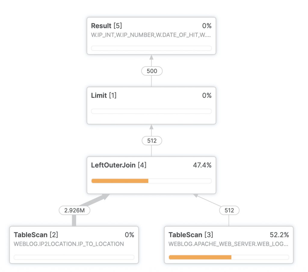
In most cases the first step in improving a Snowflake query is examining the query profiler. Here’s the query profile for the first test run of the geolocation:

The left outer join seems to be the culprit here. It turns out Snowflake’s optimizer doesn’t particularly like doing a left outer join on an inequality. The interesting thing about that is this should be a one to one relationship. For each IP number in the web log, there should be exactly one row where that IP number falls into the right range.

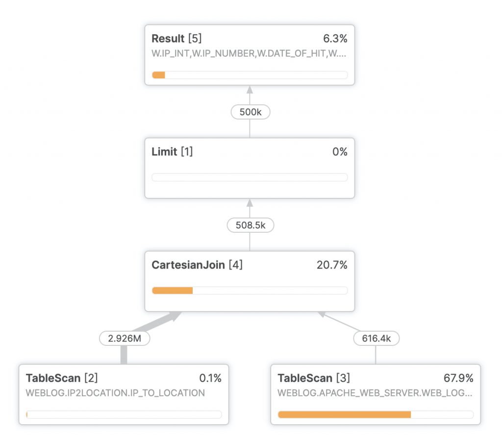
This allows us to do a cartesian join instead:

select * from "WEBLOG"."APACHE_WEB_SERVER"."WEB_LOG_ENRICHED" W
 inner join "WEBLOG"."IP2LOCATION"."IP_TO_LOCATION" L
    on W.IP_INT >= L.START_IP and W.IP_INT <= L.END_IP limit 500000;

This leads to a query profile like this:

More important, it leads to performance like this on an extra small warehouse:

After running an initial query that took a few seconds and got the critical IP geolocation table into the cache, geolocating half a million web log entries took just five seconds.

Least Privilege Access to Monitor Snowflake Usage

Posted on November 25, 2020November 25, 2020 by Greg Pavlik

The SNOWFLAKE Database

All Snowflake accounts should have a database named SNOWFLAKE. It’s a shared database, using Snowflake’s secure data sharing.

If you set up your Snowflake account before the spring of 2019, you may need to import the shared database. If you don’t see the SNOWFLAKE database in your account and don’t see it as an inbound share, contact Snowflake Support.

Snowflake, Inc. (the company) unsurprisingly runs a number of its own Snowflake accounts. The SNOWFLAKE database in your account is an inbound share from the Snowflake, Inc. account running on your cloud provider and region.

Because the SNOWFLAKE database contains information on usage and metering, by default only the ACCOUNTADMIN role has privileges to select on the views.

Attempting Grants on the SNOWFLAKE Database

Without this background, it’s possible to conclude improperly that only the ACCOUNTADMIN can access the views in the SNOWFLAKE database. Here’s why:

-- A user may try something like this:
use role ACCOUNTADMIN;
grant select on "SNOWFLAKE"."ACCOUNT_USAGE"."QUERY_HISTORY" to role SYSADMIN;

This will result in the error Grant not executed: Insufficient privileges.

The ACCOUNTADMIN is the most powerful role in a Snowflake account. Because of this, a person may conclude that there’s no way to grant privileges on the “special” SNOWFLAKE database.

Granting Privileges on SNOWFLAKE to Human Users

As previously discussed, the only thing special about the SNOWFLAKE database is it’s an inbound shared database. You can grant access to the SNOWFLAKE database the same way you do for any other inbound shared database:

use role ACCOUNTADMIN;
grant imported privileges on database SNOWFLAKE to role SYSADMIN;
use role SYSADMIN; -- Remember to always get out of the ACCOUNTADMIN role when done using it.

This will grant select on all views in the SNOWFLAKE database to the SYSADMIN role. It’s up to your organization whether or not you want to grant this access. Personally, I recommend it. It allows users with SYSADMIN role but not ACCOUNTADMIN role to monitor usage. It also allows users with ACCOUNTADMIN role to use least privilege to access this information without changing roles to ACCOUNTADMIN. Any time a user changes to ACCOUNTADMIN it’s possible to forget to get out of that role. That risks performing other actions such as creating object that generally shouldn’t be done in that role.

Granting Privileges on SNOWFLAKE to Machine Users

If granting access to the SNOWFLAKE database is for a dashboard or machine user, you can do something like this:

-- You must use the ACCOUNTADMIN role to assign the required privileges
use role ACCOUNTADMIN;
 
-- Optionally create a warehouse to monitor Snowflake activity.
-- Only create a warehouse dedicated to account usage if there are several
-- clients (performance monitors, BI packages, etc.) using it.
create or replace warehouse MONITOR_SNOWFLAKE warehouse_size = 'X-Small';
 
-- Create a new role intended to monitor Snowflake usage.
create or replace role MONITOR_SNOWFLAKE;
 
-- Grant privileges on the SNOWFLAKE database to the new role.
grant imported privileges on database SNOWFLAKE to role MONITOR_SNOWFLAKE;
 
-- Create a user.
create or replace user    SNOWFLAKE_MONITOR
    LOGIN_NAME          = SNOWFLAKE_MONITOR
    password            = 'My_Password_123!'
    default_warehouse   = MONITOR_SNOWFLAKE
    default_role        = MONITOR_SNOWFLAKE
    default_namespace   = SNOWFLAKE.ACCOUNT_USAGE
--  rsa_public_key      = 'MIIBIjANBgkqh...' -- Optional, see note.
;
 
-- Note: Snowflake recommends using key authentication for machine users:
-- https://docs.snowflake.com/en/user-guide/snowsql-start.html#using-key-pair-authentication
 
-- Grant usage on the warehouse used to monitor Snowflake.
grant usage on warehouse MONITOR_SNOWFLAKE to role MONITOR_SNOWFLAKE;
 
-- Grant the monitor role to the user.
grant role MONITOR_SNOWFLAKE to user SNOWFLAKE_MONITOR;
 
-- Get out of the ACCOUNTADMIN role when done.
use role SYSADMIN;

Increasing Granularity of the Grants

Let’s discuss more granular access to the views in an imported shared database. Privileges on the imported shared database itself are all or nothing. If you want to control access with more granularity, create a set of “select * from…” views selecting from the SNOWFLAKE database. You can then manage the grants on those views individually.

Snowflake Version

Posted on November 24, 2020November 24, 2020 by Greg Pavlik

One of the great things about being a Snowflake customer is you’ll never have to perform upgrades and patches. Snowflake performs upgrades and patches for you, transparently with no down time or degraded performance.

Upgrades and patches happen so seamlessly, I suspect most customers would have no idea what release of the Snowflake platform they’re currently running. I know I don’t. That’s a good thing. Old features keep working as Snowflake enables new features on an ongoing basis.

There are times when it’s useful to know what version of Snowflake you’re running. You can check what version of Snowflake you’re running using the CURRENT_VERSION() function:

select CURRENT_VERSION();

At the time of this writing, the current version of Snowflake is 4.39.5. There are situations where it’s useful to know when Snowflake performed upgrades and patches over time. For example, if you have a SQL statement that you didn’t change and it performed differently than before, one explanation could be a change of Snowflake version.

You can check your Snowflake version over time running this statement:

select      to_date(min(START_TIME))  as START_DATE,
            to_date(max(START_TIME))  as END_DATE,
            RELEASE_VERSION           as SNOWFLAKE_VERSION
from        "SNOWFLAKE"."ACCOUNT_USAGE"."QUERY_HISTORY"
group by    RELEASE_VERSION
having      START_DATE >= current_date - 30   -- Check upgrades for previous 30 days 
order by    START_DATE desc;

If you see a change in version between the times your regularly run statement executed differently, that could be one possibility. To help confirm that, you can go to the query history in the Snowflake UI and examine the query profiles for each query. If they look the same, the version upgrade isn’t the explanation for the difference. If they look different, the version upgrade could be a possible reason.

Regex Non-Capturing Groups and Lookarounds in Snowflake

Posted on November 20, 2020September 27, 2021 by Greg Pavlik

If you don’t need the background or discussion of how they work and just want to download Snowflake UDFs that support regex non-capturing groups, lookaheads, and lookbehinds, you can download them here:

https://github.com/GregPavlik/SnowflakeUDFs/tree/main/RegularExpressions

Now for the background:

Snowflake supports regular expressions (regex) for string matching and replacements. If your regex skills are like mine, Snowflake’s regex implementation provides more than you’ll ever need.

For regex ninjas and people who want to use regular expression libraries, there are two commonly-used capabilities that this post explains Snowflake’s regex functions do not currently support: non-capturing groups and lookarounds.

Every once in a while I run into a customer who’s a regex ninja or wants to use a regex from a library that requires one of these capabilities.

It occurred to me that JavaScript supports regex with these features, and Snowflake supports JavaScript user defined functions (UDFs). To use a regex in Snowflake that has non-capturing groups or lookarounds, It’s a simple matter of writing a UDF.

The problem is writing a new UDF for each use of a regex reduces some of the main advantages of regular expressions including compactness and simplicity.

This lead me to write two general-purpose UDFs that approximate Snowflake’s REGEXP_REPLACE and RLIKE (synonym REGEXP_LIKE) as closely as possible while enabling non-capturing groups and lookarounds.

I named the JavaScript UDFs similar to the Snowflake functions they approximate, REGEXP_REPLACE2 and RLIKE2 (synonym REGEXP_LIKE2). I also overloaded the UDFs so that you can call them using minimal parameters or optional parameters the same as their base Snowflake functions.

Here’s an example of their usage:

-- Running the base function returns this error:
-- Invalid regular expression: 'bar(?=bar)', no argument for repetition operator: ?
select regexp_replace('foobarbarfoo', 'bar(?=bar)', '***');

-- Running the UDF approximating the base function returns foo***barfoo
select regexp_replace2('foobarbarfoo', 'bar(?=bar)', '***');

-- Running the base function returns this error:
-- Invalid regular expression: 'bar(?=bar)', no argument for repetition operator: ?
select rlike('foobarbarfoo', 'bar(?=bar)');

-- Running the UDF approximating the base function returns TRUE
select rlike2('foobarbarfoo', 'bar(?=bar)');

You can download the UDFs on my Github here: https://github.com/GregPavlik/SnowflakeUDFs/tree/main/RegularExpressions

Getting Snowflake Primary Key Columns as a Table

Posted on July 29, 2020May 25, 2021 by Greg Pavlik

One of my customers had an interesting requirement. In order to dynamically create merge statements, they needed a way to collect the primary key columns for any given table. After discussing some options — returning them as a delimited string, array, etc., we agreed that returning the columns in a table is the best option.

This User Defined Table Function (UDTF) returns the columns for a table’s primary key. The UDTF will return a table with a single column, each row in the table is one of the columns in the input table’s primary key. If there is no primary key, the table will have no rows. For a single-column primary key, the table will have the one row, and for composite primary keys it will return all columns in the key.

One thing you may notice is that the input to the UDTF is the table’s DDL, not just the table’s name. The reason for this is because UDTFs cannot execute SQL. The simplest way to handle this situation is to nest the GET_DDL function as the parameter for the GET_PK_COLUMNS function. You can see how this works in the code samp

create database DB_Primary_Keys;

/**************************************************************************************************************
*                                                                                                             *
*  Set up test tables with four types of primary key: Named composite, unnamed composite, inline, and none.   * 
*                                                                                                             *
**************************************************************************************************************/
 
-- Named multi-column PK
create or replace temporary table table1
(
column_name1 number NOT NULL,
column_name2 number NOT NULL,
column_name3 string,
CONSTRAINT Constraint_name PRIMARY KEY (column_name1, column_name2)
);
 
-- Unnamed multi-column PK
create temporary table table2
(
column_name1 number NOT NULL,
column_name2 number NOT NULL,
column_name3 string,
PRIMARY KEY (column_name1, column_name2)
);
 
-- Inline single-column PK
create or replace temporary table table3
(
column_name1 number primary key,
column_name2 number NOT NULL,
column_name3 string
);
 
-- No PK defined
create or replace temporary table table4
(
column_name1 number,
column_name2 number,
column_name3 string
);
 
/********************************************************************************************************
*                                                                                                       *
* User defined table function (UDTF) to get primary keys for a table.                                   *
*                                                                                                       *
* @param  {string}:  TABLE_DDL    The DDL for the table to get the PKs. Usually use get_ddl.            *
* @return {table}:                A table with the columns comprising the table's primary key           *
*                                                                                                       *
********************************************************************************************************/
create or replace function GET_PK_COLUMNS(TABLE_DDL string)
returns table (PK_COLUMN string)
language javascript
as
$$
{
    processRow: function get_params(row, rowWriter, context){
        var pkCols = getPKs(row.TABLE_DDL);
        for (i = 0; i < pkCols.length; i++) {
            rowWriter.writeRow({PK_COLUMN: pkCols[i]}); 
        }
         
        function getPKs(tableDDL) {
            var c;
            var keyword = "primary key";
            var ins = -1;
            var s = tableDDL.split("\n");
            for (var i = 0; i < s.length; i++) {  
                ins = s[i].indexOf(keyword);
                if (ins != -1) {
                    var colList = s[i].substring(ins + keyword.length);
                    colList = colList.replace("(", "");
                    colList = colList.replace(")", "");
                    var colArray = colList.split(",");
                    for (pkc = 0; c < colArray.length; pkc++) {
                        colArray[pkc] = colArray[pkc].trim();
                    }
                    return colArray;
                }
            }
            return [];  // No PK
        }
    }
}
$$;
 
/**************************************************************************************************************
*                                                                                                             *
*  Test execution of the UDTF.                                                                                * 
*                                                                                                             *
**************************************************************************************************************/
 
select * from table(get_pk_columns(get_ddl('table', 'table1'))) PKS;  -- Multi-column PK with named constraint
select * from table(get_pk_columns(get_ddl('table', 'table2'))) PKS;  -- Multi-column PK with no name for constraint
select * from table(get_pk_columns(get_ddl('table', 'table3'))) PKS;  -- Single column PK inline definition
select * from table(get_pk_columns(get_ddl('table', 'table4'))) PKS;  -- No PKs

Oracle to Snowflake Table DDL Conversion

Posted on April 28, 2020April 28, 2020 by Greg Pavlik

Jason Trewin at FreshGravity provided this Oracle to Snowflake Table DDL conversion script. FreshGravity is a great Snowflake partner, and Jason is working on his second Snowflake deployment for our shared customers.

He shared a great approach to DDL conversion from Oracle to Snowflake. I thought it was so useful that after some discussion he agreed to let me write up and post on it.

You can modify the where clauses to select the tables you need to convert, and modify the mappings from Oracle table owners to Snowflake owners.

Thanks and credit to Jason Trewin for contributing this useful script to the Snowflake community.

-- Script contributed to the Snowflake community courtesy of Jason Trewin at FreshGravity.

SELECT 'CREATE OR REPLACE TABLE '  
        || NEW_SCHEMA_NAME
        || '.' ||  TABLE_NAME || ' (' || LISTAGG(COLUMN_NAME || ' ' || CONVERTED_DATA_TYPE || CASE WHEN NULLABLE = 'N' THEN ' NOT NULL' ELSE ''END , ' , ') WITHIN GROUP (ORDER BY COLUMN_ID)  || ');' --AS COLUMN_LIST
   FROM (      
 SELECT DATA_TYPE, COLUMN_NAME, ALL_TABLES.TABLE_NAME, ALL_TABLES.OWNER,DATA_LENGTH, DATA_PRECISION, DATA_SCALE, NULLABLE,
        CASE WHEN INSTR(DATA_TYPE,'WITH LOCAL TIME ZONE') > 0  THEN 'TIMESTAMP_TZ'
             WHEN INSTR(DATA_TYPE,'TIMESTAMP') > 0 THEN 'TIMESTAMP_NTZ'
             WHEN DATA_TYPE = 'DATE' THEN 'DATE'
             WHEN DATA_TYPE = 'XMLTYPE' THEN 'VARIANT'
             WHEN DATA_TYPE IN ('BINARY_DOUBLE','NUMBER') THEN 'NUMBER'||
                  CASE WHEN DATA_PRECISION IS NOT NULL THEN  '('|| DATA_PRECISION || ',' || NVL(DATA_SCALE,0) || ')'
                            ELSE '' END
             WHEN DATA_TYPE IN ('NVARCHAR2','VARCHAR2','VARCHAR','NVARCHAR') THEN 'TEXT(' || DATA_LENGTH  || ')'
             WHEN DATA_TYPE IN ('NCHAR','CHAR') THEN 'TEXT(1)'
             WHEN DATA_TYPE = 'CLOB' THEN 'TEXT(16777216)'
             ELSE NULL END AS CONVERTED_DATA_TYPE
             ,CASE WHEN ALL_TABLES.OWNER = 'ORACLE_OWNER_1' THEN 'SNOWFLAKE_OWNER_1'  -- Map Oracle owners to Snowflake owners.
                   WHEN ALL_TABLES.OWNER = 'ORACLE_OWNER_2' THEN 'SNOWFLAKE_OWNER_2'
                   WHEN ALL_TABLES.OWNER = 'ORACLE_OWNER_3' THEN 'SNOWFLAKE_OWNER_3'                                      
                   WHEN ALL_TABLES.OWNER = 'ORACLE_OWNER_4' THEN 'SNOWFLAKE_OWNER_4'
				   WHEN ALL_TABLES.OWNER = 'ORACLE_OWNER_5' THEN 'SNOWFLAKE_OWNER_5'  
                   WHEN ALL_TABLES.OWNER = 'ORACLE_OWNER_6' THEN 'SNOWFLAKE_OWNER_6'                                      
               ELSE NULL END AS NEW_SCHEMA_NAME
             ,COLUMN_ID
  FROM ALL_TAB_COLUMNS
       INNER JOIN ALL_TABLES   
          ON ALL_TABLES.TABLE_NAME  =  ALL_TAB_COLUMNS.TABLE_NAME
         AND ALL_TABLES.OWNER       =  ALL_TAB_COLUMNS.OWNER
WHERE	-- Insert a where clause to decide which tables to include or exclude. This is just part of one approach: 
	ALL_TABLES.TABLE_NAME NOT IN ('TABLE1','TABLE2','TABLE3')
  )
GROUP BY NEW_SCHEMA_NAME, TABLE_NAME



SELECT TEXT_LINE FROM (
SELECT 1 AS INDEXING_VALUE,
     TABLE_NAME ,
     OWNER,
        'CREATE OR REPLACE TABLE '  
        || CASE WHEN ALL_TABLES.OWNER = 'ORACLE_OWNER_1' THEN 'SNOWFLAKE_OWNER_1'  		-- Map Oracle table ownwers to Snowflake table owners
                WHEN ALL_TABLES.OWNER = 'ORACLE_OWNER_2' THEN 'SNOWFLAKE_OWNER_2'
                WHEN ALL_TABLES.OWNER = 'ORACLE_OWNER_3' THEN 'SNOWFLAKE_OWNER_3'                                      
                WHEN ALL_TABLES.OWNER = 'ORACLE_OWNER_4' THEN 'SNOWFLAKE_OWNER_4'
                WHEN ALL_TABLES.OWNER = 'ORACLE_OWNER_5' THEN 'SNOWFLAKE_OWNER_5'  
                WHEN ALL_TABLES.OWNER = 'ORACLE_OWNER_6' THEN 'SNOWFLAKE_OWNER_6'                                      
           ELSE NULL END         || '.' ||  TABLE_NAME || '(' AS TEXT_LINE, 1 AS COLUMN_ID
  FROM ALL_TABLES   
WHERE ALL_TABLES.OWNER LIKE 'ORACLE_OWNER_%'	-- Set where condition for tables to process.
AND ALL_TABLES.TABLE_NAME IN ('TABLE1', 'TABLE2', 'TABLE3')
UNION ALL
SELECT 2  AS INDEXING_VALUE, ALL_TABLES.TABLE_NAME , ALL_TABLES.OWNER,
        CASE WHEN COLUMN_ID = 1 THEN '' ELSE ',' END || COLUMN_NAME || ' ' ||
            CASE WHEN INSTR(DATA_TYPE,'WITH LOCAL TIME ZONE') > 0  THEN 'TIMESTAMP_TZ'
             WHEN INSTR(DATA_TYPE,'TIMESTAMP') > 0 THEN 'TIMESTAMP_NTZ'
             WHEN DATA_TYPE = 'DATE' THEN 'DATE'
             WHEN DATA_TYPE = 'XMLTYPE' THEN 'VARIANT'
             WHEN DATA_TYPE IN ('BINARY_DOUBLE','NUMBER') THEN 'NUMBER'||
                  CASE WHEN DATA_PRECISION IS NOT NULL THEN  '('|| DATA_PRECISION || ',' || NVL(DATA_SCALE,0) || ')'
                            ELSE '' END
             WHEN DATA_TYPE IN ('NVARCHAR2','VARCHAR2','VARCHAR','NVARCHAR') THEN 'TEXT(' || DATA_LENGTH  || ')'
             WHEN DATA_TYPE IN ('NCHAR','CHAR') THEN 'TEXT(1)'
             WHEN DATA_TYPE = 'CLOB' THEN 'TEXT(16777216)'
             ELSE NULL END ||  CASE WHEN NULLABLE = 'N' THEN ' NOT NULL' ELSE ''END  AS CONVERTED_DATA_TYPE
           ,COLUMN_ID
  FROM ALL_TAB_COLUMNS
       INNER JOIN ALL_TABLES   
          ON ALL_TABLES.TABLE_NAME  =  ALL_TAB_COLUMNS.TABLE_NAME
         AND ALL_TABLES.OWNER       =  ALL_TAB_COLUMNS.OWNER
WHERE ALL_TABLES.OWNER LIKE 'ODS_%'
AND ALL_TABLES.TABLE_NAME IN ('TABLE1', 'TABLE2', 'TABLE3') 
 UNION ALL SELECT 3 AS INDEXING_VALUE,
     TABLE_NAME , OWNER,
        ');', 1 AS COLUMN_ID
  FROM ALL_TABLES   
WHERE ALL_TABLES.OWNER LIKE 'ORACLE_OWNER_%'
AND ALL_TABLES.TABLE_NAME IN ('TABLE1', 'TABLE2', 'TABLE3')
)
ORDER BY TABLE_NAME, OWNER, INDEXING_VALUE, COLUMN_ID



SELECT  'ALTER TABLE '
        || CASE WHEN ALL_TABLES.OWNER = 'ORACLE_OWNER_1' THEN 'SNOWFLAKE_OWNER_1'  		-- Map Oracle table ownwers to Snowflake table owners
                WHEN ALL_TABLES.OWNER = 'ORACLE_OWNER_2' THEN 'SNOWFLAKE_OWNER_2'
                WHEN ALL_TABLES.OWNER = 'ORACLE_OWNER_3' THEN 'SNOWFLAKE_OWNER_3'                                      
                WHEN ALL_TABLES.OWNER = 'ORACLE_OWNER_4' THEN 'SNOWFLAKE_OWNER_4'
                WHEN ALL_TABLES.OWNER = 'ORACLE_OWNER_5' THEN 'SNOWFLAKE_OWNER_5'  
                WHEN ALL_TABLES.OWNER = 'ORACLE_OWNER_6' THEN 'SNOWFLAKE_OWNER_6'                                       
           ELSE NULL END         || '.' ||  TABLE_NAME
        || ' ADD PRIMARY KEY (' ||PK_COLUMMN_LIST || ');'
FROM 
 (
SELECT --'ALTER TABLE ' 
       COLS.OWNER, COLS.TABLE_NAME, LISTAGG(cols.COLUMN_NAME , ',') WITHIN GROUP (ORDER BY POSITION) AS PK_COLUMMN_LIST
--       cols.table_name, cols.column_name, cols.POSITION, cons.owner
FROM all_constraints cons, all_cons_columns cols
WHERE cols.OWNER LIKE 'ORACLE_OWNER_%'
AND cons.constraint_type = 'P'
AND cons.constraint_name = cols.constraint_name
AND cons.owner = cols.owner
GROUP BY  COLS.OWNER, COLS.TABLE_NAME
)

Overloading JavaScript UDFs in Snowflake

Posted on April 11, 2020April 14, 2020 by Greg Pavlik

Snowflake supports overloading user defined functions. It’s a great way to handle function calls with parameters of different data types or different numbers of parameters. Developers often overload functions to let users send only relevant parameters.

Consider the common SUBSTRING function. You can call it using one of two overloads:

select substr('Hello, world.', 8);     --This returns "world."

select substr('Hello, world.', 8, 5);  --This returns "world"

In the first statement, the caller sent the string to use and the start position. Omitting the final parameter uses the overload with default behavior, returning to the end of the string.

In the second statement, the caller decided to get rid of the final period. Adding the third parameter for length used the other overload to return five characters instead of the default behavior.

This is a common design with overloaded functions. Mandatory parameters go on the left and optional parameters follow. Each allowable combination of parameters becomes an overload of the function. In this design, developers typically write one base function with all parameters. For the overloads with missing parameters, they’ll call the base function using a default value for the missing parameter(s).

This design ensures that there’s only one place to maintain and debug code. The problem is Snowflake JavaScript UDFs cannot call other UDFs. While one way to deal with this is to write the same code in all overloads, it means three places to maintain, improve, and debug code. Fortunately, there’s a way to write once base function and call it from overloaded functions using defaults.

The solution is to write the base UDF with all parameters in JavaScript. For the overloads that simply call the base function using defaults for missing parameters, call the base JavaScript UDF using an overloaded SQL UDF. This works because SQL UDFs can call other UDFs, which JavaScript UDFs cannot do.

In this example, the JavaScript UDF returns a column displaying a graphical progress bar. The opens are typical for progress bars: percent completion, number of decimal places to display on the percentage, and number of segments to display.

The only one that can’t be defaulted is the percent complete. It’s okay to default to two decimal points and ten segments.

-- Make a progress bar function that looks like this:   ⬛⬛⬜⬜⬜⬜⬜⬜⬜⬜ 24.53%

-- This is the main JavaScript function with all parameters.
create or replace function PROGRESS_BAR(PERCENTAGE float, DECIMALS float, SEGMENTS float)
returns string
language javascript
as
$$

    var percent = PERCENTAGE;
    
    if (isNaN(percent)) percent =   0;
    if (percent < 0)    percent =   0;
    if (percent > 100)  percent = 100;

    percent        = percent.toFixed(DECIMALS);

    var filledSegments = Math.round(SEGMENTS * (percent / 100));
    var emptySegments  = SEGMENTS - filledSegments;

    var bar = '⬛'.repeat(filledSegments) + '⬜'.repeat(emptySegments);
 
    return bar + " " + percent + "%";

$$;

-- This is an overload with only the percentage, using defaults for 
-- number of segments and decimal points to display on percentage.
create or replace function PROGRESS_BAR(PERCENTAGE float)
returns string
language sql
as
$$
    select progress_bar(PERCENTAGE, 2, 10)
$$;

-- This is an overload with the percentage and the option set for the
-- number of decimals to display. It uses a default for number of segments.
create or replace function PROGRESS_BAR(PERCENTAGE float, DECIMALS float)
returns string
language sql
as
$$
    select progress_bar(PERCENTAGE, DECIMALS, 10)
$$;

-- Call the main JavaScript function by sending all three parameters:
select progress_bar(24.5293, 0, 100) as PROGRESS;

-- Call the overloaded SQL function by omitting the number of segments (segments defaults to 10):
select progress_bar(24.5293, 1) as PROGRESS;

-- Call the overloaded SQL function specifying only the percentage 
-- (segments defaults to 10 and decimals to 2)
-- It should display like this:   ⬛⬛⬜⬜⬜⬜⬜⬜⬜⬜ 24.53%
select progress_bar(24.5293) as PROGRESS;

By the way, this UDF progress bar is fully functional. If you have a long-running process such as loading a large number of files, you can use it to monitor progress by refreshing the query periodically. Here’s an example using a long progress bar and 24.41%:

select progress_bar(24.41, 2, 100) as PROGRESS;